Can a playback EQ perfectly cancel a cutting EQ?
Can a Playback EQ Perfectly Cancel a Cutting EQ?
The question this page answers: Do the cutting-side EQ (cutting EQ) and the playback-side EQ (phono preamp) perfectly cancel each other when combined? This page goes deep into the residuals visible in real-unit pairs through simulation, the theory and implementations of perfect cancellation, and the essence of the "±2 dB tolerance" lying beyond.
A note up front
This page does not set out to settle which curve to play records back with. This FAQ assumes the same RIAA curve as defined by the three time constants 75 / 318 / 3180 μs. For the basics of "where do the LCR / RC / NF naming and circuit-topology differences come from", see the sister FAQ Are LCR and RC Phono Equalizers Fundamentally Different?.
This page goes further from there, drawing on simulation: what happens when you cascade the cutting EQ and the playback EQ, whether a playback EQ that perfectly cancels exists, and what residuals appear in the historically-attested real-unit pairs.
This is a separate topic from "whether you can hear it", and it is also independent of the curve-disagreement debate.
Bottom line first
To set out short answers to the questions that come up repeatedly in this FAQ:
Premise: with the same time constants, LCR and RC are mathematically equivalent — indistinguishable in both amplitude and phase. This was covered in detail in the sister FAQ Are LCR and RC Phono Equalizers Fundamentally Different?. Building on that, the two questions this page addresses:
- A playback EQ that perfectly cancels a specific cutting EQ does exist in theory. For the ideal RIAA curve, you can implement a perfectly canceling playback EQ even with passive L, C, R elements only, using the constant-resistance bridged-T topology systematized by O. J. Zobel in his 1928 Bell System Technical Journal paper (details in §3).
- However, in the historically-attested real-unit pairs of cutting and playback, additional poles/zeros and stage-configuration differences mean that perfect cancellation does not occur. Up to about 3 dB in amplitude and a 100°-scale spread in phase from +14° to -101° (including sign reversal) remain near 20 kHz (details in §1 and §2).
The rest of this page walks through the simulation that leads to these conclusions, step by step.
1. Simulation results: LCR-type cutting EQ × RC/NF-type playback EQ
The author simulated the cutting-side (preemphasis) and playback-side (phono preamp) phono EQ circuits using a small-signal linear-equivalent model in LTspice.
First, let's look at the cutting-side preemphasis curves.
For the ideal RIAA simulation, LTspice's transfer-function description was used to write H(s) directly from the three time constants (3180 µs / 318 µs / 75 µs), without any circuit elements — i.e., the theoretical curve itself.
For the Neumann SE-66 simulation, the schematic posted on Pspatial Audio was redrawn in LTspice (op-amp, single stage + auxiliary circuitry).
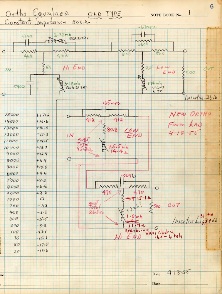
For the rare hand-drawn schematic that RCA Victor used when cutting New Orthophonic discs (dated 1955-04-18, RCA engineering notebook 1, p.6), Nicholas Bergh kindly provided the source, and the circuit was redrawn in LTspice. This hand-drawn schematic has also been confirmed equivalent to the redraw dated 1957-02-07 by R. McLaughlin.
According to Nicholas Bergh, the major cutting-EQ manufacturers of the 1950s split into two lineages: LCR type (Cinema Engineering / Westrex) and RC type (Gotham / Neumann). Both are first-order, and the RCA New Orthophonic in this simulation corresponds to the LCR type. Nick has pointed out that a small difference around 800 Hz may emerge between the two lineages, but as the simulation results below indicate, the principal driver of cascade residuals in the scope of this FAQ is not the cutting-side LCR/RC difference but rather the playback-side circuit-topology difference (NF vs CR) combined with the additional poles and zeros specific to each implementation.
The frequency-response curves of these three implementations — Neumann SE-66, RCA New Orthophonic 1955-57, and the ideal RIAA — overlaid on a single plot, look like this:
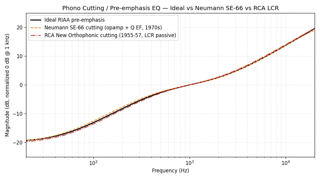
All three follow the ideal RIAA closely, with implementation-to-implementation differences within 1 dB even at the band edges.
Next, let's look at the playback-side phono preamp curves.
For the playback side (phono preamp), the Luxman CL35/III and the Marantz 7C were reconstructed in LTspice by reading the schematics in their service manuals of the time (the theoretical RIAA was written down using LTspice's transfer-function description as the inverse of the cutting side, just as on the cutting side).
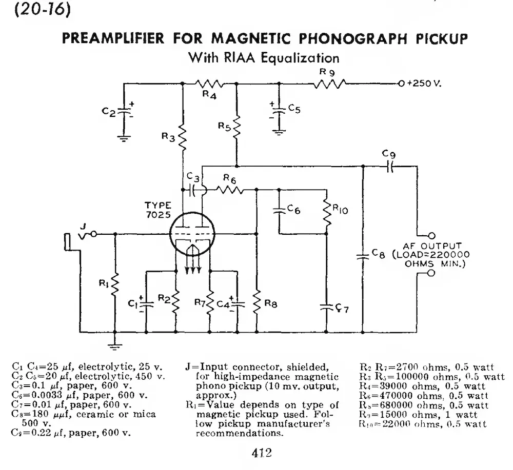
The RCA 1960 CR type was reconstructed in LTspice from the phono preamp schematic on p.412 of the RCA Receiving Tube Manual RC-20 (1960) (TYPE 7025 + interstage RC EQ, passive type) (the schematic is shown later).
The frequency-response curves of these four implementations — Luxman CL35/III, Marantz 7C, RCA 1960 CR type (the circuit shown in RC-20), and the ideal RIAA — overlaid on a single plot, look like this:
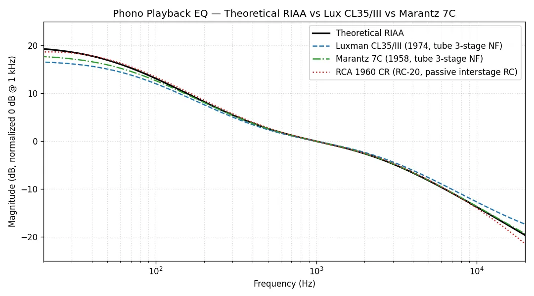
All four roughly follow the ideal RIAA inverse characteristic, but the Luxman CL35/III's high end runs noticeably shallower than the theoretical value, and its low end sits a bit lower as well. The RCA 1960 CR and the Marantz 7C are nearly identical to the theoretical.
Ideally, since these two — the cutting (recording)-side equalizer and the playback-side equalizer — are inverses of each other, cascading them should cancel out into a flat response (0 dB / 0°). Because of small implementation-to-implementation differences, however, the cascade response is not perfectly flat, and residuals appear at the band edges.
This is fundamentally the same phenomenon as the spread observed in the 21-unit measurement survey of the 1972 Stereo Sound magazine, covered in Pt.23 §23.1. While Pt.23 §23.1 demonstrated the spread through measurements on real units, this simulation shows that the same spread can be explained theoretically from differences in circuit topology.
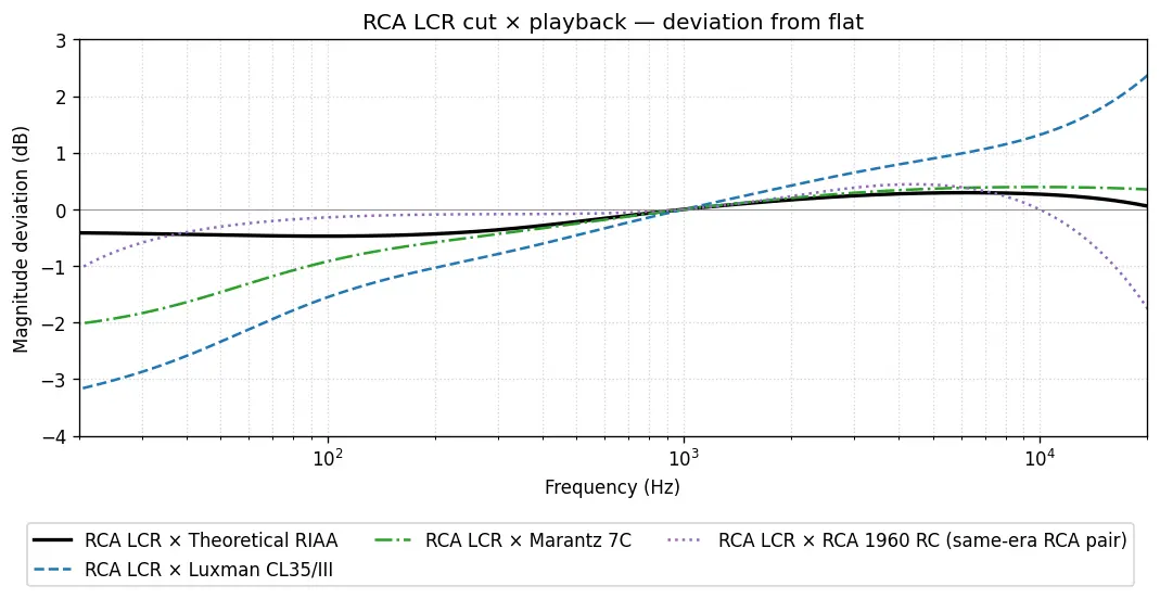
Cascade results combining cutting side and playback side
Concretely, fixing the cutting side as a presumed reconstruction of the mid-1950s RCA lateral cutting EQ (constant impedance 500 Ω, an LCR passive configuration using inductors), the cascade residuals when combined with four playback phono preamps, with 1 kHz as the 0 dB / 0° reference, are tabulated below (for the definitions of NF type / CR type, see §2.2 of the sister FAQ Are LCR and RC Phono Equalizers Fundamentally Different?):
| cutting × playback | 20 Hz | 10 kHz | 20 kHz |
|---|---|---|---|
| theoretical RIAA preemphasis × theoretical RIAA playback (reference) | 0.00 dB / 0° | 0.00 / 0° | 0.00 / 0° |
| 1950s RCA LCR × RCA 1960 CR type | -1.06 / +32.8° | 0.00 / -28.4° | -1.73 / -53.6° |
| 1950s RCA LCR × Marantz 7C (1958, NF type) | -2.02 / +1.4° | +0.39 / -3.4° | +0.35 / -4.6° |
| 1950s RCA LCR × Luxman CL35/III (1974, NF type) | -3.18 / +6.7° | +1.32 / +6.1° | +2.35 / +13.7° |
What stands out is that the residual phase around 20 kHz for the same LCR cutting changes sign depending on the category of the playback-side circuit topology:
- CR type (RCA 1960, the circuit shown in RC-20): -53.6°
- NF type (Marantz 7C): -4.6°
- NF type (Luxman CL35/III): +13.7°
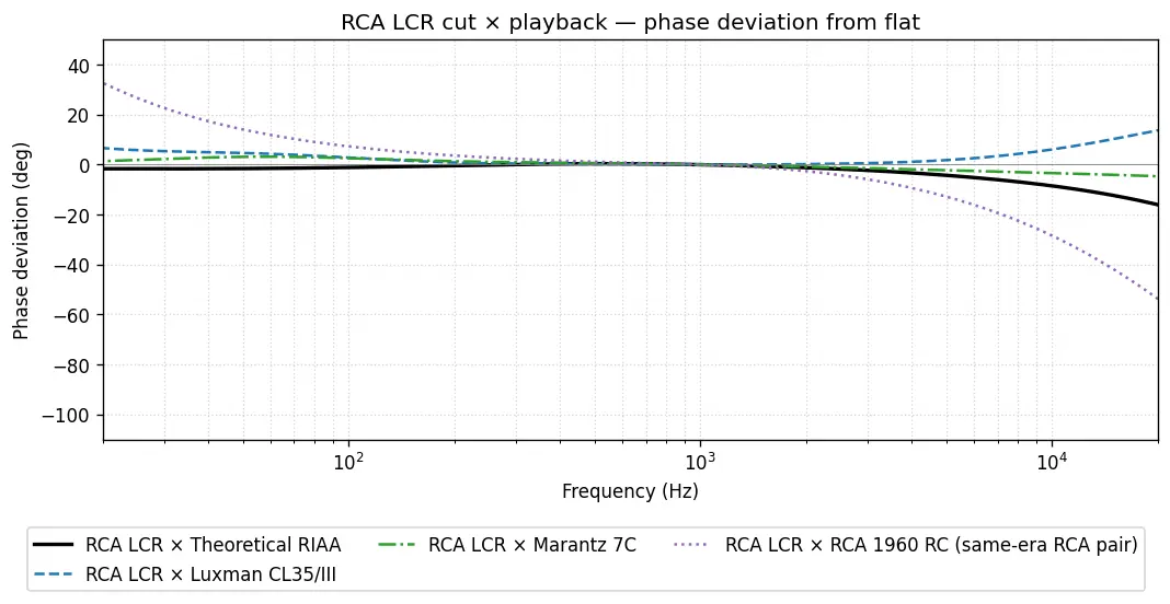
What is interesting is that even the CR type — which RCA consistently recommended in its own official publications throughout the 22 years from 1953 (Moyer, "Evolution of a Recording Curve," Audio Engineering magazine) to 1975 (Receiving Tube Manual series final edition RC-30) as the playback side for the RIAA curve — leaves a non-trivial 20 kHz phase residual of -53.6°. Even when both the cutting and playback sides come from the same manufacturer and the same era — a combination of RCA-family implementations — full cancellation does not occur.
2. Simulation results: RC-type cutting EQ × RC/NF-type playback EQ
Up to this point, the cutting side was fixed at the mid-1950s RCA LCR cutting EQ. So what happens to the cascade residuals when the cutting side is replaced with the 1970s Neumann SE-66 (an op-amp single-stage + auxiliary-circuit RC-based implementation)?
Here, "RC-type cutting EQ" refers to an implementation that uses no inductors on the cutting side and is built from op-amps and RC networks (such as the Neumann SE-66). This is a classification by whether L is included or not, on a different axis from the playback-side "CR type / NF type" subdivision introduced in §2.2 of the sister FAQ.
| cutting × playback | 20 Hz | 10 kHz | 20 kHz |
|---|---|---|---|
| theoretical RIAA preemphasis × theoretical RIAA playback (reference) | 0.00 dB / 0° | 0.00 / 0° | 0.00 / 0° |
| Neumann SE-66 × theoretical RIAA playback | -0.04 / +7.3° | -0.03 / -27.7° | -0.60 / -63.7° |
| Neumann SE-66 × Marantz 7C (NF type) | -1.65 / +10.3° | +0.10 / -22.6° | -0.31 / -52.4° |
| Neumann SE-66 × Luxman CL35/III (NF type) | -2.80 / +15.6° | +1.02 / -13.2° | +1.70 / -34.0° |
| Neumann SE-66 × RCA 1960 CR type | -0.68 / +41.8° | -0.30 / -47.6° | -2.39 / -101.3° |
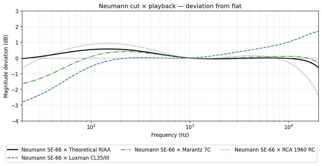
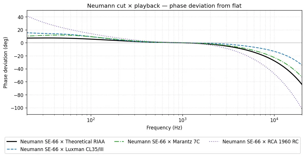
What is striking is that even when the cutting side is changed to the RC-based Neumann SE-66, the phase residual around 20 kHz still varies considerably with the playback-side circuit topology. In particular, the Neumann SE-66 × RCA 1960 CR type combination shows a residual of about -101° at 20 kHz, which is substantially larger even than the -54° shown above for the 1950s RCA LCR × RCA 1960 CR type combination.
This result suggests that the working understanding that originally launched this simulation effort — "if you play back an LCR-cut record through RC, the phases don't line up", which Nicholas Bergh and the author had been discussing by email — can be sharpened further from a simulation standpoint. At least within the implementation set covered by this simulation, the principal driver of the differences in the residuals is, more than the cutting-side LCR-vs-RC distinction itself, the combination of the playback-side circuit-topology difference (NF type vs CR type) and the additional poles and zeros specific to each implementation, as observed in the data. The result departed substantially from what was initially expected, and the author is keenly aware that this finding will require further reflection and additional investigation.
3. Does a playback EQ that perfectly cancels a cutting EQ exist in theory?
Looking at the simulation results above, the following question naturally arises. For a given cutting EQ, does a playback EQ that mathematically cancels its frequency and phase response exactly exist in theory? This section answers the question in four steps, building on what this simulation has shown. This is one step away from the central question of this FAQ (whether real-world cutting/playback combinations align in phase); §3.4 returns to the main thread.
3.1 Mathematically, it must exist
In the finite-order, lumped-parameter linear circuit model considered here, the frequency response in the complex frequency s domain is a rational function H(s) = K · Π(1+s·τ_z) / Π(1+s·τ_p). Its inverse 1/H(s) is a rational function of the same form with zeros and poles swapped, and can also always be written down. In other words, "the transfer characteristic of a playback EQ that mathematically cancels the cutting EQ exactly" can always be written down on paper.
However, whether this inverse transfer characteristic behaves as a stable and causal physical circuit, and whether it can be realized with passive elements only, are separate conditions, addressed respectively in §3.2 (behavioral-source implementation) and §3.3 (passive LCR implementation) below.
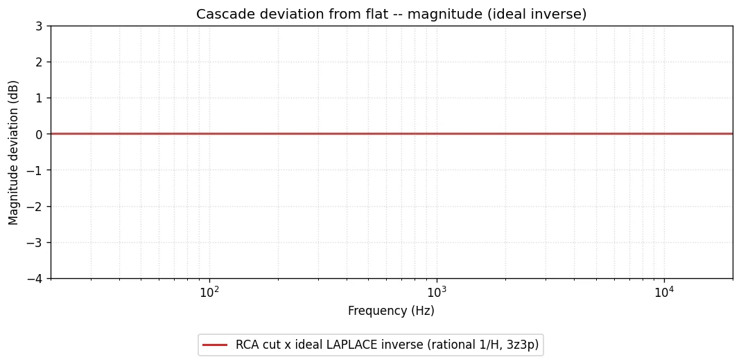
3.2 With a behavioral source, the simulation cancels it completely
Using LTspice's Laplace-transform description, one can place 1/H(s) directly into a circuit as a behavioral source. In this simulation, the RCA New Orthophonic LCR cutting EQ was approximated by a rational-function fit (3 zeros, 3 poles) and its inverse implemented as a Laplace source. The cascade of the cutting EQ with this Laplace inverse is perfectly flat at 0.000 dB / 0.00° (within the limits of floating-point precision) across all frequencies.
3.3 Even passive LCR can implement it via textbook methods
Even when the condition "passive elements (L, C, R) only, no behavioral source" is added, the standard RIAA playback EQ can be implemented exactly using a circuit topology systematized by O. J. Zobel in his 1928 Bell System Technical Journal paper ("Distortion Correction in Electrical Circuits with Constant Resistance Recurrent Networks", Vol. 7, No. 3) — the constant-resistance bridged-T. In this simulation, sympy was used to derive the design equations symbolically, and the auto-generated passive LCR netlist gave the following component values:
- Low-frequency stage (3180 µs pole / 318 µs zero): bridge arm L=1.7172 H paralleled with R=5.4 kΩ; shunt arm C=4.77 µF in series with R=66.67 Ω
- High-frequency stage (75 µs pole): bridge arm L=45 mH (pure L); shunt arm C=0.125 µF (pure C)
- 600 Ω matched-impedance termination on both input and output
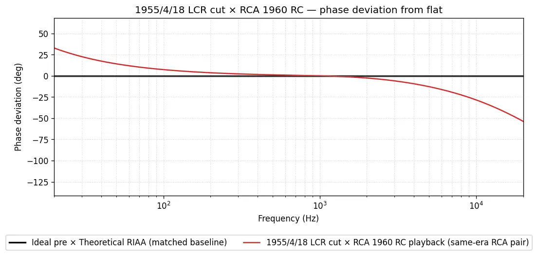
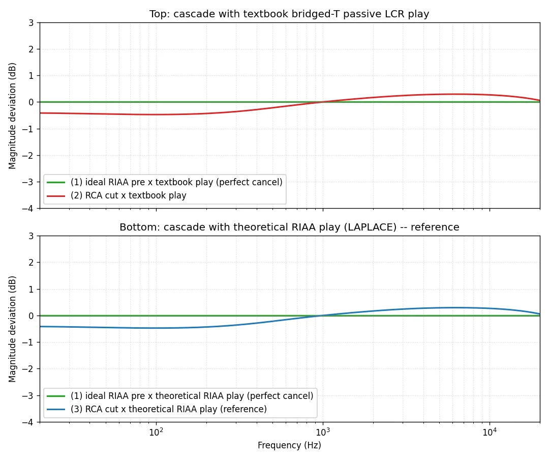
The figure below has two panels: the upper panel shows the cascade using this passive LCR playback EQ, and the lower panel (reference) shows the cascade using the ideal playback EQ implemented with the Laplace source from the previous subsection. The green line (combination with the ideal RIAA preemphasis) stays at 0 dB in both panels, and the colored line (combination with the RCA New Orthophonic cutting EQ) takes nearly the same shape in both panels.
The colored line deviates from 0 dB by up to about ±0.5 dB, and the deviation is also visually noticeable. However, this stems from the fact that the RCA New Orthophonic cutting EQ itself deviates from the ideal RIAA, not from any imprecision of the passive LCR playback EQ implementation. The fact that they appear in the same shape in both panels is what shows that the textbook-designed passive LCR achieves the same characteristic as the theoretical ideal playback EQ (Laplace version).
The passive LCR phono-preamp coils and units, such as Hashimoto Electric's H-EQL still available today, or the now-discontinued Okamoto Laboratory's LCR-1A (component values documented in Matsunami Kikatsu's article in the May 1989 issue of MJ Musen-to-Jikken, a Japanese DIY audio magazine), also adopt this constant-resistance bridged-T two-stage cascade structurally. Real units use minor approximations imposed by component-value availability (e.g., the standard value 5.3 µF) and other implementation constraints, with manufacturer-stated deviations of about ±0.1 to ±0.5 dB (for example, the Hashimoto Electric H-EQL datasheet specifies ±0.1 dB for the recommended circuit No.1 and ±0.4 dB for the trimmed versions No.2 / No.3). Implementing the theoretical values from this simulation would yield a deviation on the order of ±0.0001 dB, but that is a matter of purpose.
3.4 "Implementation accuracy" and "phase alignment in real-world cutting/playback pairs" are separate questions
Sections 3.1 through 3.3 above showed that for the pair "a specific theoretical cutting EQ and the playback EQ that perfectly cancels it", the simulation can achieve perfect cancellation.
In actual record playback, however, the cutting side carries subtly different implementations of the RIAA curve depending on the studio, era, and cutting equipment (this simulation also covered the difference between RCA New Orthophonic and Neumann SE-66), and the playback-side phono preamp adds its own poles and zeros depending on its circuit topology and design choices (the multi-implementation comparison in §1 and §2 of this simulation).
And as repeatedly shown in §1 and §2, even within RIAA, the cascade of real-world (i.e., historically attested) cutting and playback designs shows up to about 3 dB in amplitude and a 100°-scale spread in phase from +14° to -101° around 20 kHz, including sign reversal. Reflecting on the simulation as a whole, the unvarnished impression is that for ordinary record cutting and playback (phono preamp implementation) pairs, perfect alignment of both frequency and phase response is extremely rare (except for the mathematically-existing ideal pair).
Whether the residual phase is audible is a separate point. For that, see §5.1 and the separate page Can you hear a difference when you change the EQ curve?.
4. Limitations of the simulation model
The simulations above treat tubes and passive elements with a small-signal linear-equivalent model. Specifically:
- Tubes are represented by the three-parameter linear model μ (gain) / r_p (internal resistance) / g_m (transconductance)
- The input signal is small-amplitude and linear only around the operating point
- Large-signal distortion, output clipping, power-supply ripple, thermal behavior, and tube-to-tube variation are not included
Within this scope, what can be seen is frequency response (amplitude and phase) only. Judgments about "sound quality" are not included. Real units involve nonlinear operation, component tolerances, and loading conditions with the cartridge, and they do not match the simulation perfectly.
Note that the simulation also does not include the transfer characteristics of the cutter head or playback cartridge themselves. However, according to Lipshitz et al.'s 1980 preprint:
"Disk cutter heads and modern wide-band pickup cartridges have been found to exhibit simple minimum-phase behaviour to beyond 20 kHz, even including whatever resonances and mechanical breakup modes may occur below this upper limit."
— Lipshitz, S. P., Pocock, M., & Vanderkooy, J., "Preliminary Results on the Audibility of Midrange Phase Distortion in Audio Systems", 67th AES Convention Preprint #1714, 1980, p.10
In other words, even when these mechanical stages are included, the framework of the §3 "perfect cancellation of EQ networks" argument — rational-function representation of minimum-phase systems and its inverse — remains valid.
Also, of the combinations shown in §1 and §2, most fall within the RIAA ±2 dB tolerance, but some — such as the Luxman CL35/III at -3.18 dB at 20 Hz, and the Neumann SE-66 × RCA 1960 CR type at -2.39 dB at 20 kHz — fall outside the tolerance at the band edges. None of these is "wrong"; each shows the characteristic difference of its respective implementation.
5. How to read this (independence from audibility and other arguments)
5.1 Whether this is audible is a separate question
The numbers -53.6° or +13.7° for the residual phase around 20 kHz are measurements of frequency response, not direct claims about audible difference. For the discussion of how sensitive the human auditory system is to high-frequency phase shifts, see the separate page Can you hear a difference when you change the EQ curve?.
This separation of "the electrical characteristic and audibility are separate questions" rests on a long-standing body of work in the AES (Audio Engineering Society) literature. Lipshitz et al. (1982), one of the representative experimental papers on the audibility of phase distortion, states in §2:
"The high-frequency rolloff is generally almost phase linear over the passband, whereas the low-frequency rolloff is accompanied by considerable phase distortions. Much available research indicates that the high-frequency phase nonlinearity is innocuous (...). What concerns us more is phase distortion occurring between these frequency extremes, say, from 100 Hz to 3 kHz—what we shall refer to as midrange phase distortion in this paper. It is in this area that most researchers have found that the ear's sensitivity to phase distortion is greatest."
— Lipshitz, S. P., Pocock, M., & Vanderkooy, J., "On the Audibility of Midrange Phase Distortion in Audio Systems", Journal of the Audio Engineering Society, Vol.30 No.9, September 1982, p.585
The summary §5 of the same paper states:
"Phase distortions accompany many links in the audio chain. The most frequent manifestations of these phase nonlinearities occur near the low- and high-frequency cutoffs of the system, where significant differential time delays occur. At these extreme frequencies, however, the bulk of the evidence indicates that quite sizable phase distortions are inaudible."
— Ibid., p.593
That said, the paper's primary experimental subject is midrange phase distortion (100 Hz to 3 kHz) in loudspeaker systems, not the residual phase of phono preamps near 20 kHz. The -101° to +14° residuals observed in this FAQ fall within what Lipshitz et al. call "extreme frequencies," and the paper's general line of argument leans toward classifying such cases as inaudible — but the paper does not directly or explicitly demonstrate inaudibility for this band.
Furthermore, in the 1980 preprint that preceded their 1982 paper, Lipshitz, Pocock, and Vanderkooy themselves cautioned:
"All the effects described can reasonably be classified as subtle. We are NOT, in our present state of knowledge, advocating that phase linear transducers are a requirement for high-quality sound reproduction. More research is necessary."
— Lipshitz, S. P., Pocock, M., & Vanderkooy, J., "Preliminary Results on the Audibility of Midrange Phase Distortion in Audio Systems", 67th AES Convention Preprint #1714, 1980, p.24
Further, when Shanefield commented that "phase distortion in practical systems appears to be of negligible importance" (JAES 31(6), 1983, p.447) — after compiling negative evidence from blind tests of music played over loudspeakers — the authors closed their reply with "We are basically in agreement with Dr. Shanefield" (Authors' Reply, JAES 31(6), 1983, p.448). The authors themselves thus framed the practical importance of phase distortion in normal loudspeaker playback as small.
5.2 Independent from the "cut with non-RIAA curves" view
What this FAQ addresses is the residual phase due to differences in implementation circuit topology, assuming the same time constants (75 / 318 / 3180 μs). By contrast, the view that "American stereo LPs are cut with non-RIAA curves" claims that the time constants themselves are different. The two are independent discussions, and the simulation results in this FAQ are neither evidence for nor against such a view.
Specifically:
- The residual phase due to the playback-side circuit topology is, in principle, a different thing from the target one tries to home in on by switching time constants with a variable EQ. The former is a difference among first-order RC implementations sharing the same time constants; the latter implies a difference in the time constants themselves
- The presence of a residual phase is no evidence that a different time constant was used at cutting time
- The roughly 3 dB spread in amplitude and the 100°-scale spread in phase from +14° to -101°, including sign reversal, are also observed — within the implementation set covered in this simulation — as implementation differences within first-order operation, derived from the pole/zero structure of the transfer function
A separate page summarizes the curve-disagreement debate: Are American stereo LPs cut with the RIAA curve?.
6. Read further
- For the basics of "what is the difference between LCR type and RC type": sister FAQ "Are LCR and RC Phono Equalizers Fundamentally Different?"
- For the wording transition in standards documents from LCR to RC: When did the standards documents change their wording for the time constants from LCR to all-RC?
- For the details and discovery story behind the Nick figure in §1: Phono EQ Curves Liner Notes I
- Blog series Pt.23: §23.1 covers the 21-unit measurement survey of the 1972 Stereo Sound magazine (measured spread in phase and amplitude); §23.2 quotes Nicholas Bergh's (ARSC/AES) email of December 2022
Closing
To close, let's look back at what came into view through this simulation as a single narrative.
In the actual cascades, more often than not, residuals appeared beyond what was expected, which was surprising. The initial guess was just "if you play back an LCR-cut record through RC, the phases don't line up", but in practice, even an RC-cut record played back through an RC preamp produced phase residuals on the order of 100° around 20 kHz, depending on the combination.
So can perfect cancellation never happen? As covered in §3, it turns out that for a specific theoretical pair, perfect cancellation is achievable mathematically, in simulation with a Laplace behavioral source, and even in textbook passive LCR designs. The constant-resistance bridged-T topology systematized by Zobel in 1928 is precisely the circuit topology for that purpose.
But cutting EQs and playback EQs come in many implementation flavors. Studio by studio, era by era, piece of equipment by piece of equipment, there are differences in additional poles/zeros and stage configurations. As a result, the additional poles/zeros differ for each cutting-side implementation, and the degree of cancellation also varies depending on the playback EQ implementation.
Seen this way, the ±2 dB tolerance in the RIAA standard might take on a meaning beyond a mere measurement-error buffer — perhaps "a margin built into the standard to accommodate the differences that inevitably arise when the same target curve is approximated by diverse physical implementations". Reflecting on the simulation as a whole, that is at least how it appears to the author.
Whether this is audible, and if so where in the soundstage or timbre it acts, is in the territory of listening experiments and psychoacoustics. This FAQ is no more than the entrance to that open question.
Revision History
- May 18, 2026: Added quotes in §5.1 from Lipshitz et al.'s 1980 preprint caution and the 1983 Shanefield comment with authors' reply, and in §4 from Lipshitz et al.'s 1980 preprint on cutter head / cartridge minimum-phase behavior
- May 15, 2026: Adjusted the paragraph order at the start of §2
- May 13, 2026: Initial publication